Serial and Parallel Regions

Overview

Teaching: 15 min
Exercises: 5 min

Questions

• What is a good parallel algorithm?

Objectives

• Introduce theoretical concepts relating to parallel algorithms.

• Describe theoretical limitations on parallel computation.

Serial and Parallel Execution

An algorithm is a series of steps to solve a problem. Let us imagine these steps as a familiar scene in car manufacturing:

• Each step adds or adjusts a component to an existing structure to form a car as the conveyor belt moves.
• As a designer of these processes, you would carefully order the way you add components so that you don’t have to disassemble already constructed parts.
• How long does it take to build a car in this way?

Now, you would like to build cars faster since there are impatient customers waiting in line! What do you do? You build two lines of conveyor belts and hire twice number of people to do the work. Now you get two cars in the same amount of time!

• If your problem can be solved like this, you are in luck. You just need more CPUs (or cores) to do the work.
• This is called an “Embarrassingly Parallel (EP)” problem and is the easiest problem to parallelize.

But what if you’re a boutique car manufacturer, making only a handful of cars, and constructing a new assembly line would cost more time and money than it would save? How can you produce cars more quickly without constructing an extra line? The only way is to have multiple people work on the same car at the same time:

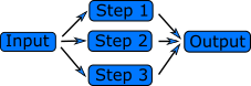
• You identify the steps which don’t interfere with each other and can be executed at the same time (e.g., the front part of the car can be constructed independently of the rear part of the car).
• If you find more steps which can be done without interfering with each other, these steps can be executed at the same time.
• Overall time is saved. More cars for the same amount of time!

In this case, the most important thing to consider is the independence of a step (that is, whether a step can be executed without interfering with other steps). This independency is called “atomicity” of an operation.

In the analogy with car manufacturing, the speed of conveyor belt is the “clock” of CPU, parts are “input”, doing something is an “operation”, and the car structure on the conveyor belt is “output”. The algorithm is the set of operations that constructs a car from the parts.
It consists of individual steps, adding parts or adjusting them. These could be done one after the other by a single worker.

If we want to produce a car faster, maybe we can do some of the work in parallel. Let’s say we can hire four workers to attach each of the tires at the same time. All of these steps have the same input, a car without tires, and they work together to create an output, a car with tires. The crucial thing that allows us to add the tires in parallel is that they are independent. Adding one tire does not prevent you from adding another, or require that any of the other tires are added. The workers operate on different parts of the car.

Data Dependency

Another example, and a common operation in scientific computing, is the calculation of quantities that evolve in time or in an otherwise iterative manner (e.g. molecular dynamics, gradient descent). A simple implementation might look like this:

old_value = starting_point
for iteration in 1 ... 10000
   new_value = function(old_value)
   old_value = new_value

This is a very bad parallel algorithm! Every step, or iteration of the for loop, depends on the value of the previous step.

The important factor that determines whether steps can be run in parallel is data dependencies. In our example above, every step depends on data from the previous step, the value of the old_value variable. When attaching tires to a car, attaching one tire does not depend on attaching the others, so these steps can be done at the same time.

However, attaching the front tires both require that the axis is there. This step must be completed first, but the two tires can then be attached at the same time.

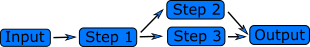
A part of the program that cannot be run in parallel is called a “serial region” and a part that can be run in parallel is called a “parallel region”. Any program will have some serial regions. In a good parallel program, most of the time is spent in parallel regions. The program can never run faster than the sum of the serial regions.

Serial and Parallel regions

Identify serial and parallel regions in the following algorithm

 vector_1[0] = 1;
 vector_1[1] = 1;
 for i in 2 ... 1000
   vector_1[i] = vector_1[i-1] + vector_1[i-2];

 for i in 0 ... 1000
   vector_2[i] = i;

 for i in 0 ... 1000
   vector_3[i] = vector_2[i] + vector_1[i];
   print("The sum of the vectors is.", vector_3[i]);

Solution

serial   | vector_0[0] = 1;
         | vector_1[1] = 1;
         | for i in 2 ... 1000
         |   vector_1[i] = vector_1[i-1] + vector_1[i-2];

parallel | for i in 0 ... 1000
         |   vector_2[i] = i;

parallel | for i in 0 ... 1000
         |   vector_3[i] = vector_2[i] + vector_1[i];
         |   print("The sum of the vectors is.", vector_3[i]);

The first and the second loop could also run at the same time.

In the first loop, every iteration depends on data from the previous two. In the second two loops, nothing in a step depends on any of the other steps.

Scalability

The speedup when running a parallel program on multiple processors can be defined as

where $t_1$ is the computational time for running the software using one processor, and $t_N$ is the computational time running the same software with N processors.

• Ideally, we would like software to have a linear speedup that is equal to the number of processors (speedup = N), as that would mean that every processor would be contributing 100% of its computational power.
• Unfortunately, this is a very challenging goal for real applications to attain.

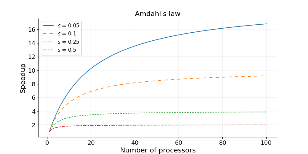
Amdahl’s Law and strong scaling

There is a theoretical limit in what parallelization can achieve, and it is encapsulated in “Amdahl’s Law”:

where $s$ is the proportion of execution time spent on the serial part, $p$ is the proportion of execution time spent on the part that can be parallelized, and $N$ is the number of processors. Amdahl’s law states that, for a fixed problem, the upper limit of speedup is determined by the serial fraction of the code. This is called strong scaling and its consequences can be understood from the figure below.

Amdahl’s law in practice

Consider a program that takes 20 hours to run using one core. If a particular part of the program, which takes one hour to execute, cannot be parallelized (s = 1/20 = 0.05), and if the code that takes up the remaining 19 hours of execution time can be parallelized (p = 1 − s = 0.95), then regardless of how many processors are devoted to a parallelized execution of this program, the minimum execution time cannot be less than that critical one hour. Hence, the theoretical speedup is limited to at most 20 times (when N = ∞, speedup = 1/s = 20).

Strong scaling

• Defined as how the solution time varies with the number of processors for a fixed total problem size.
• Linear strong scaling if the speedup (work units completed per unit time) is equal to the number of processing elements used.
• Harder to achieve good strong-scaling at larger process counts since communication overhead typically increases with the number of processes used.

In practice the sizes of problems scale with the amount of available resources, and we also need a measure for a relative speedup which takes into account increasing problem sizes.

Gustafson’s law and weak scaling

Gustafson’s law is based on the approximations that the parallel part scales linearly with the amount of resources, and that the serial part does not increase with respect to the size of the problem. It provides a formula for scaled speedup:

where $s$, $p$ and $N$ have the same meaning as in Amdahl’s law. With Gustafson’s law the scaled speedup increases linearly with respect to the number of processors (with a slope smaller than one), and there is no upper limit for the scaled speedup. This is called weak scaling, where the scaled speedup is calculated based on the amount of work done for a scaled problem size (in contrast to Amdahl’s law which focuses on fixed problem size).

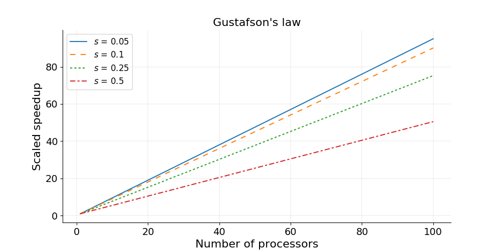
Weak scaling

• Defined as how the solution time varies with the number of processors for a fixed problem size per processor.
• Linear weak scaling if the run time stays constant while the workload is increased in direct proportion to the number of processors.

Communication considerations

The other significant factors in the speed of a parallel program are communication speed and latency.

• Communication speed is determined by the amount of data one needs to send/receive, and the bandwidth of the underlying hardware for the communication.
• Latency consists of the software latency (how long the operating system needs in order to prepare for a communication), and the hardware latency (how long the hardware takes to send/receive even a small bit of data).

For a fixed-size problem, the time spent in communication is not significant when the number of ranks is small and the execution of parallel regions gets faster with the number of ranks. But if we keep increasing the number of ranks, the time spent in communication grows when multiple cores are involved with communication

Surface-to-Volume Ratio

In a parallel algorithm, the data which is handled by a core can be considered in two parts: the part the CPU needs that other cores control, and a part that the core controls itself and can compute. The whole data which a CPU or a core computes is the sum of the two. The data under the control of the other cores is called “surface” and the whole data is called “volume”.

The surface data requires communications. The more surface there is, the more communications among CPUs/cores is needed, and the longer the program will take to finish.

Due to Amdahl’s law, you want to minimize the number of communications for the same surface since each communication takes finite amount of time to prepare (latency). This suggests that the surface data be exchanged in one communication if possible, not small parts of the surface data exchanged in multiple communications. Of course, sequential consistency should be obeyed when the surface data is exchanged.

Further reading

• Strong and weak scaling

Key Points

• Algorithms can have parallelisable and non-parallelisable sections.

• A highly parallel algorithm may be slower on a single processor.

• The theoretical maximum speed is determined by the serial sections.

• The other main restriction is communication speed between the processes.