Parallel Paradigms and Parallel Algorithms

Overview

Teaching: 20 min
Exercises: 0 min

Questions

• How do I split the work?

Objectives

• Introduce Message Passing and Data Parallel.

• Introduce Parallel Algorithm.

• Introduce standard communication and data storage patterns.

Parallel Paradigms

How to achieve a parallel computation is divided roughly into two paradigms.

• One is “data parallel” and the other is “message passing”.
• MPI (Message Passing Interface) clearly belongs to the second paradigm.
• “OpenMP” is based on “data parallelism”

Message passing vs data parallelism

• In the message passing paradigm, each CPU (or core) runs an independent program.

• Parallelism is achieved by receiving data which it doesn’t have, and sending data which it has.

• In the data parallel paradigm, there are many different data and the same operations (instructions in assembly language) are performed on these data at the same time.
• Parallelism is achieved by how many different data a single operation can act on.

This division is mainly due to historical development of parallel architectures: one follows from shared memory architecture like SMP (Shared Memory Processor) and the other from distributed computer architecture. A familiar example of the shared memory architecture is GPU (or multi-core CPU) architecture and a familiar example of the distributed computing architecture is a cluster computer. Which architecture is more useful depends on what kind of problems you have. Sometimes, one has to use both!

Consider a simple loop which can be sped up if we have many cores for illustration:

do i=1,N

  a(i) = b(i) + c(i)

enddo

for(i=0; i<N; i++) {

  a[i] = b[i] + c[i];

}

for i in range(N):
    a[i] = b[i] + c[i]

If we have $N$ or cores, each element of the loop can be computed in just one step (for a factor of $N$ speed-up).

Data Parallel

One standard method for programming in data parallel fashion is called “OpenMP” (for “Open MultiProcessing”).

To understand what data parallel means, let’s consider the following bit of OpenMP code which parallelizes the above loop:

!$omp parallel do
do i=1,N

  a(i) = b(i) + c(i)

enddo

To understand what data parallel means, let’s consider the following bit of OpenMP code which parallelizes the above loop:

#pragma omp parallel for
for(i=0; i<N; i++) {

  a[i] = b[i] + c[i];

}

• Parallelization achieved by just one additional line, handled by the preprocessor in the compile stage.
• Possible since the computer system architecture supports OpenMP and all the complicated mechanisms for parallelization are hidden.
• Means that the system architecture has a shared memory view of variables and each core can access all of the memory address.
• The compiler “calculates” the address off-set for each core and let each one compute on a part of the whole data.

Here, the catch word is shared memory which allows all cores to access all the address space.

In Python, process-based parallelism is supported by the multiprocessing module.

Message Passing

In the message passing paradigm, each processor runs its own program and works on its own data. To work on the same problem in parallel, they communicate by sending messages to each other. Again using the above example, each core runs the same program over a portion of the data. For example:

do i=1,m

  a(i) = b(i) + c(i)

enddo

for(i=0; i<m; i++) {

  a[i] = b[i] + c[i];

}

for i in range(m):
    a[i] = b[i] + c[i]

• Other than changing the number of loops from N to m, the code is exactly the same.
• m is the reduced number of loops each core needs to do (if there are N cores, m is 1 (= N/N)).

But the parallelization by message passing is not complete yet. In the message passing paradigm, each core is independent from the other cores.

• Must make sure that each core has correct data to compute and write out the results in correct order.
• Depends on the computer system.
• For example in a cluster computer, sometimes only one core has an access to the file system. This core reads in the whole data and sends the correct data to each core (including itself). MPI communications!
• After the computation, each core sends the result to that particular core, which core writes out the received data in a file in the correct order.
• If the cluster computer supports a parallel file system, each core reads the correct data from one file, computes and writes out the result to one file in correct order.

In the end, both data parallel and message passing logically achieve the following:

Each rank operates on its own set of data. In some cases, one has to combine the “data parallel” and “message passing” methods. For example, there are problems larger than one GPU can handle. Then, data parallelism is used for the portion of the problem contained within one GPU, and then message passing is used to employ several GPUs (each GPU handles a part of the problem) unless special hardware/software supports multiple GPU usage.

Algorithm Design

Designing a parallel algorithm that determines which of the two paradigms above one should follow rests on the actual understanding of how the problem can be solved in parallel. This requires some thought and practice.

To get used to “thinking in parallel”, we discuss “Embarrassingly Parallel” (EP) problems first and then we consider problems which are not EP problems.

Embarrassingly Parallel Problems

Problems which can be parallelized most easily are EP problems, which occur in many Monte Carlo simulation problems and in many big database search problems. In Monte Carlo simulations, random initial conditions are used in order to sample a real situation. So, a random number is given and the computation follows using this random number. Depending on the random number, some computation may finish quicker and some computation may take longer to finish. And we need to sample a lot (like a billion times) to get a rough picture of the real situation. The problem becomes running the same code with a different random number over and over again! In big database searches, one needs to dig through all the data to find wanted data. There may be just one datum or many data which fit the search criterion. Sometimes, we don’t need all the data which satisfies the condition. Sometimes, we do need all of them. To speed up the search, the big database is divided into smaller databases, and each smaller databases are searched independently by many workers!

Queue Method

Each worker will get tasks from a predefined queue (a random number in a Monte Carlo problem and smaller databases in a big database search problem). The tasks can be very different and take different amounts of time, but when a worker has completed its tasks, it will pick the next one from the queue.

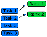
In an MPI code, the queue approach requires the ranks to communicate what they are doing to all the other ranks, resulting in some communication overhead (but negligible compared to overall task time).

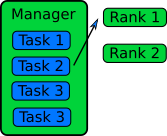
Manager / Worker Method

The manager / worker approach is a more flexible version of the queue method. We hire a manager to distribute tasks to the workers. The manager can run some complicated logic to decide which tasks to give to a worker. The manager can also perform any serial parts of the program like generating random numbers or dividing up the big database. The manager can become one of the workers after finishing managerial work.

In an MPI implementation, the main function will usually contain an if statement that determines whether the rank is the manager or a worker. The manager can execute a completely different code from the workers, or the manager can execute the same partial code as the workers once the managerial part of the code is done. It depends on whether the managerial load takes a lot of time to finish or not. Idling is a waste in parallel computing!

Because every worker rank needs to communicate with the manager, the bandwidth of the manager rank can become a bottleneck if administrative work needs a lot of information (as we can observe in real life). This can happen if the manager needs to send smaller databases (divided from one big database) to the worker ranks. This is a waste of resources and is not a suitable solution for an EP problem. Instead, it’s better to have a parallel file system so that each worker rank can access the necessary part of the big database independently.

General Parallel Problems (Non-EP Problems)

As we discussed in the 2nd lesson, in general not all the parts of a serial code can be parallelized. So, one needs to identify which part of a serial code is parallelizable. In science and technology, many numerical computations can be defined on a regular structured data (e.g., partial differential equations in a 3D space using a finite difference method). In this case, one needs to consider how to decompose the domain so that many cores can work in parallel.

Domain Decomposition

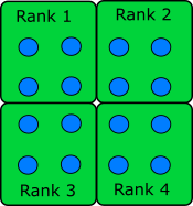
When the data is structured in a regular way, such as when simulating atoms in a crystal, it makes sense to divide the space into domains. Each rank will handle the simulation within its own domain.

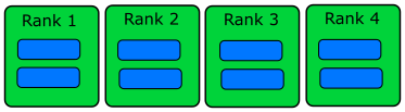
Many algorithms involve multiplying very large matrices. These include finite element methods for computational field theories as well as training and applying neural networks. The most common parallel algorithm for matrix multiplication divides the input matrices into smaller submatrices and composes the result from multiplications of the submatrices. If there are four ranks, the matrix is divided into four submatrices.

If the number of ranks is higher, each rank needs data from one row and one column to complete its operation.

Load Balancing

Even if the data is structured in a regular way and the domain is decomposed such that each core can take charge of roughly equal amounts of the sub-domain, the work that each core has to do may not be equal. For example, in weather forecasting, the 3D spatial domain can be decomposed in an equal portion. But when the sun moves across the domain, the amount of work is different in that domain since more complicated chemistry/physics is happening in that domain. Balancing this type of loads is a difficult problem and requires a careful thought before designing a parallel algorithm.

Communication Patterns

In MPI parallelization, several communication patterns occur.

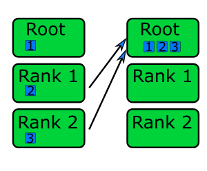
Gather / Scatter

In gather communication, all ranks send a piece of information to one rank. Gathers are typically used when printing out information or writing to disk. For example, each could send the result of a measurement to rank 0 and rank 0 could print all of them. This is necessary if only one rank has access to the screen. It also ensures that the information is printed in order.

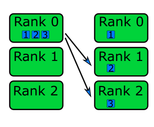
Similarly, in a scatter communication, one rank sends a piece of data to all the other ranks. Scatters are useful for communicating parameters to all the ranks doing the computation. The parameter could be read from disk but it could also be produced by a previous computation.

Gather and scatter operations require more communication as the number of ranks increases. The amount of messages sent usually increases logarithmically with the number of ranks. They have efficient implementations in the MPI libraries.

Halo Exchange

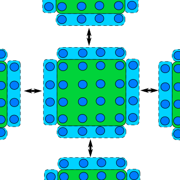
A common feature of a domain decomposed algorithm is that communications are limited to a small number of other ranks that work on a domain a short distance away. For example, in a simulation of atomic crystals, updating a single atom usually requires information from a couple of its nearest neighbours.

In such a case each rank only needs a thin slice of data from its neighbouring rank and send the same slice from its own data to the neighbour. The data received from neighbours forms a “halo” around the ranks own data.

Reduction

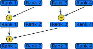
A reduction is an operation that reduces a large amount of data, a vector or a matrix, to a single number. The sum example above is a reduction. Since data is needed from all ranks, this tends to be a time consuming operation, similar to a gather operation. Usually each rank first performs the reduction locally, arriving at a single number. They then perform the steps of collecting data from some of the ranks and performing the reduction on that data, until all the data has been collected. The most efficient implementation depends on several technical features of the system. Fortunately many common reductions are implemented in the MPI library and are often optimised for a specific system.

All-to-All

In other cases, some information needs to be sent from every rank to every other rank in the system. This is the most problematic scenario; the large amount of communication required reduces the potential gain from designing a parallel algorithm. Nevertheless the performance gain may be worth the effort if it is necessary to solve the problem quickly.

Pattern Examples

The examples in the three episodes so far are also examples of different communication patterns. Can you identify one or more pattern in each example?

Key Points

• Two major paradigms, message passing and data parallel.

• MPI implements the Message Passing paradigm.

• Several standard patterns: Trivial, Queue, Master / Worker, Domain Decomposition, All-to-All.